Quantum Fourier Transform(QFT) is the quantum analogue of the discrete Fourier Transform on qubits. QFT is useful for some algorithms, like Shor's algorithm, quantum counting, etc. This will give a different perspective to understand the difference between quantum and classical algorithm.
Begin with the discrete Fourier Transform, the input data is \(x_0, x-1, \cdots, x_{N-1}\). The output is \(y_0, y_1, \cdots, y_{N-1}\), defined as follows
\[y_{k} = \frac{1}{\sqrt{N}}\sum_{j=0}^{N-1}x_{j}e^{\frac{2i\pi jk}{N}}\]
After applying Quantum Fourier Transform to the orthonormal basis |0>, |1>, ... , |j>, ... , |N-1>, the output is a superposition of states where each state represents a frequency component of the input. When |j> is the input state, the output after acting on QFT is as follows
\[QFT|j> = \frac{1}{\sqrt{N}}\sum_{k=0}^{N-1}e^{\frac{2i\pi jk}{N}}|k>\]
When an arbitrary quantum state is acted on QFT, the output is given by
\[QFT|\Phi> = QFT\sum_{j=0}^{N-1}x_{j}|j> = \frac{1}{\sqrt{N}}\sum_{j=0}^{N-1}\sum_{k=0}^{N-1}x_{j}e^{\frac{2i\pi jk}{N}}|k>\]
We have \(y_k = \frac{1}{\sqrt{N}}\sum_{j=0}^{N-1}x_{j}e^{\frac{2i\pi jk}{N}}\), then
\[QFT|\Phi> = \sum_{k=0}^{N-1}y_k|k>\]
In quantum computing, the binary representation of a number is useful for operations like QFT, which allows for efficient computation and manipulation of numbers. In binary representation, a number can be expressed as a sequence of bits, where each bit can be either 0 or 1, and each position in the sequence represents a different power of 2. The number j is represented as \(j_1j_2...j_n\), then \(j=j_12^{n-1} + j_22^{n-2} + ... + j_n2^0\). The quantum state \(|j> = |j_1j_2 ... j_{n}>\). In the other notation, \(0.j_1j_2...j_n\) is represented as \(\frac{j_1}{2^1} + \frac{j_2}{2^2} + ... + \frac{j_n}{2^n}\). We can get the representation a superposition of states on a binary sequence as follows
\[\sum_{k=0}^{N-1}|k> = \sum_{k_1=0}^{1}\cdots\sum_{k_n=0}^{1}|k_1...k_n>\]
\[k = \sum_{l=1}^{n}k_l2^{n-l} \\ \frac{k}{N} = \sum_{l=1}^{n}k_l2^{-l}\]
We discuss the output after QFT applies |j>,
\[\begin{align} |j> &\xrightarrow{QFT} \frac{1}{\sqrt{N}}\sum_{k=0}^{N-1}e^{\frac{2i\pi jk}{N}}|k> \\ &= \frac{1}{\sqrt{N}}\sum_{k_1=0}^{1}\cdots\sum_{k_n=0}^{1}e^{2i\pi j\sum_{l=1}^{n}k_l2^{-l}}|k_1...k_n> \\ &= \frac{1}{\sqrt{N}}\sum_{k_1=0}^{1}\cdots\sum_{k_n=0}^{1}\bigotimes_{l=1}^{n}e^{2i\pi jk_l2^{-l}}|k_l> \\ &= \frac{1}{\sqrt{N}}\bigotimes_{l=1}^{n}\sum_{k_l=0}^{1}e^{2i\pi jk_l2^{-l}}|k_l> \\ &= \frac{1}{\sqrt{N}}\bigotimes_{l=1}^{n}(|0> + e^{2i\pi j2^{-l}}|1>) \\ \end{align} \]
We know \(j=j_12^{n-1} + j_22^{n-2} + \cdots + j_n2^{0}\), then
\[\begin{align} e^{2i\pi j2^{-l}} &= e^{2i\pi (j_12^{n-1} + j_22^{n-2} + \cdots + j_n2^{0})2^{-l}} \\ &= e^{2i\pi (j_12^{n-1-l} + j_22^{n-2-l} + \cdots + j_n2^{-l})} \\ &= e^{2i\pi (j_{n-l+1}2^{-1} + j_{n-l+2}2^{-2} + \cdots + j_n2^{-l})} \\ &= e^{2i\pi (0.j_{n-l+1}j_{n-l+2}\cdots j_n)} \\ \end{align}\]
\[\begin{align} |j> &\xrightarrow{QFT} \frac{1}{\sqrt{N}}\bigotimes_{l=1}^{n}(|0> + e^{2i\pi j2^{-l}}|1>) \\ &= \frac{1}{\sqrt{N}}\bigotimes_{l=1}^{n}(|0> + e^{2i\pi (0.j_{n-l+1}j_{n-l+2}\cdots j_n)}|1>) \\ &= \frac{1}{\sqrt{N}}(|0> + e^{2i\pi0.j_n}|1>)(|0> + e^{2i\pi0.j_{n-1}j_n}|1>) \cdots (|0> + e^{2i\pi0.j_1j_2\cdots j_n}|1>) \end{align} \]
We note that the order of qubits,
\[ |q_0> \xrightarrow{} (|0> + e^{2i\pi0.j_n}|1>)\]
\[ |q_1> \xrightarrow{} (|0> + e^{2i\pi0.j_{n-1}j_n}|1>)\]
\[ |q_{n-1}> \xrightarrow{} (|0> + e^{2i\pi0.j_1j_2\cdots j_n}|1>)\]
We introduce a quantum gate \(R_k\), as we only want to change the phase of |1>.
\[R_k = \begin{pmatrix} 1 & 0 \\ 0 & e^{\frac{2i\pi}{2^k}} \end{pmatrix} \]
The quantum gate Controlled \(R_k\),
\[CR_k = \begin{pmatrix} 1 & 0 & 0 & 0 \\ 0 & 1 & 0 & 0 \\ 0 & 0 & 1 & 0 \\ 0 & 0 & 0 & e^{\frac{2i\pi}{2^k}} \end{pmatrix} \]
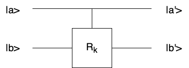
When |a> = |0>, |b'> = |b>
Wehn |a> = |1>, \(|b'> = e^{\frac{2i\pi}{2^k}}|b>\)
\[\begin{align} |b'> &= e^{\frac{2i\pi a}{2^k}}|b> = e^{2i\pi 0.\overbrace{00\cdots0}^{k-1}a}|b> \\ \end{align} \]
\[\]
I will introduce the quantum circuits for QFT. How is the procedure of QFT is explained in detail in several steps.
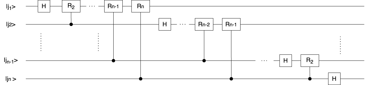
The quantum state \(|\phi_1>\)after acting a H gate on the first qubit when the input state \(|j_1j_2\cdots j_{n}>\).
\[\begin{align} |\phi_1> &= H_0|j_1j_2\cdots j_{n}> \\ &= \frac{1}{\sqrt{2}}(|0> + (-1)^{j_1}|1>)|j_2\cdots j_{n}> \\ &= \frac{1}{\sqrt{2}}(|0> + e^{2i\pi 0.j_1}|1>)|j_2\cdots j_{n}> \end{align} \]
The quantum state \(|\phi_2>\) after acting a \(CR_2\) where the first qubit is target qubit and second qubit is control qubit.
\[|\phi_2> = \frac{1}{\sqrt{2}}(|0> + e^{2i\pi 0.j_1j_2}|1>)|j_2\cdots j_{n}> \]
When \(CR_3, CR_4, ... , CR_n\) are applied, the output of the quantum state
\[|\phi_n> = \frac{1}{\sqrt{2}}(|0> + e^{2i\pi 0.j_1j_2\cdots j_{n}}|1>)|j_2\cdots j_{n}>\]
We continue to apply a H gate, \(CR_2, CR_3, ..., CR_{n-1}\) on the second qubit \(|j_2>\) in the circuit, the output of quantum state,
\[\frac{1}{\sqrt{2^2}}(|0> + e^{2i\pi 0.j_1j_2\cdots j_{n}}|1>)(|0> + e^{2i\pi 0.j_2\cdots j_{n}}|1>)|j_3\cdots j_{n}>\]
The final quantum state of the QFT circuit,
\[\frac{1}{\sqrt{N}}(|0> + e^{2i\pi 0.j_1j_2\cdots j_{n}}|1>)(|0> + e^{2i\pi 0.j_2\cdots j_{n}}|1>)\cdots (|0> + e^{2i\pi 0.j_{n}}|1>)\]
However, we need to note the first qubit \((|0> + e^{2i\pi 0.j_{n}}|1>)\) mentioned above. Then 1st and nth qubit, 2nd and (n-1)th qubit, ..., jth and (n-1-j)th qubit, are switched. We can get the final circuit of QFT as follows
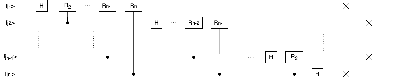
\[\frac{1}{\sqrt{N}}(|0> + e^{2i\pi 0.j_{n}}|1>)\cdots(|0> + e^{2i\pi 0.j_2\cdots j_{n}}|1>)(|0> + e^{2i\pi 0.j_1j_2\cdots j_{n}}|1>)\]
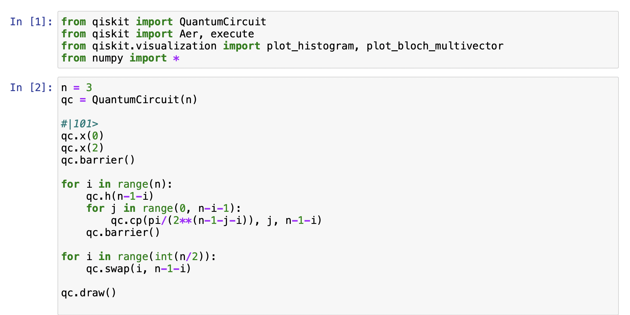
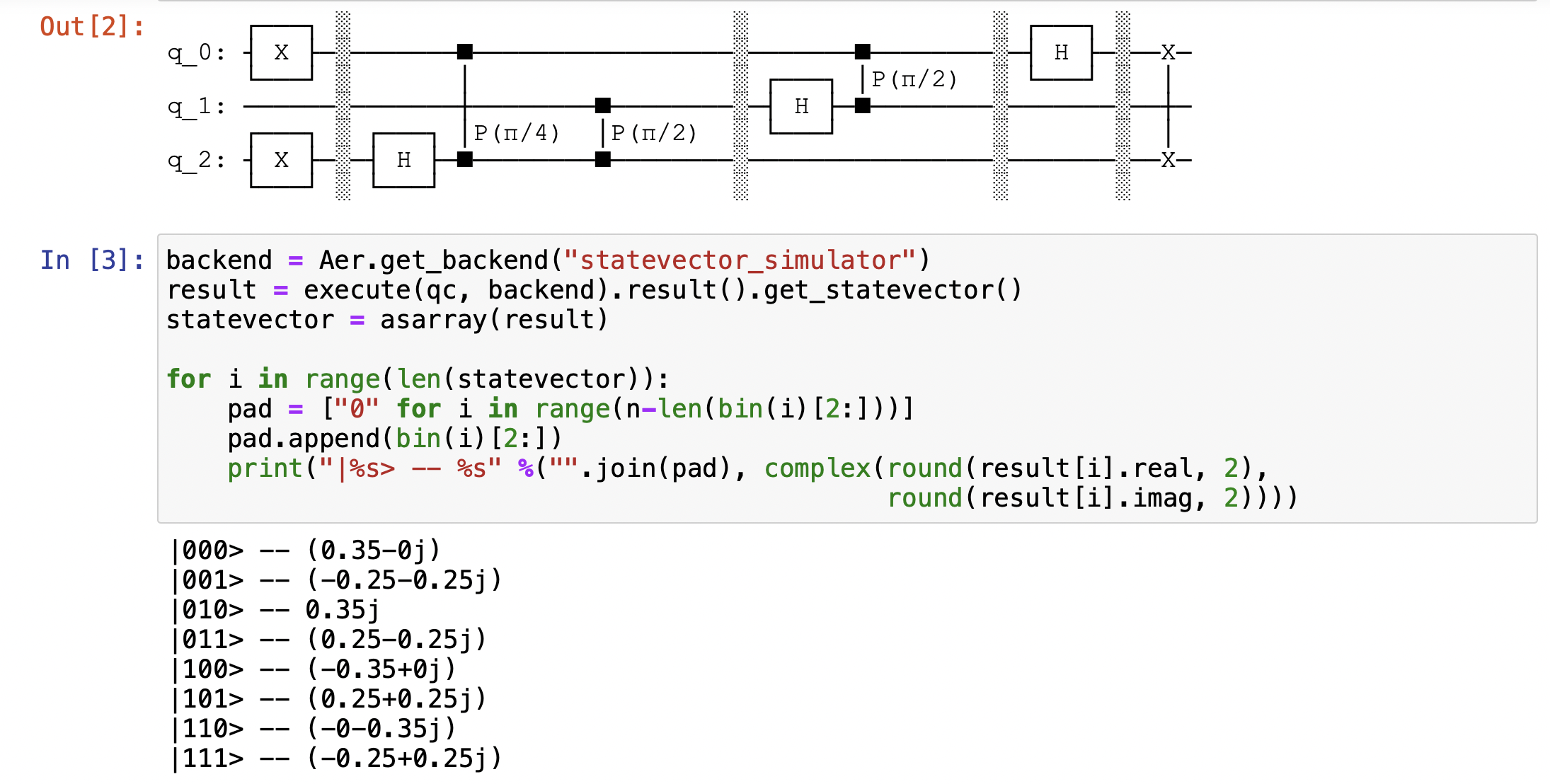
Example on Qiskit
We can use 3 qubit of QFT and the input |101> for explaining the accuracy of the quantum circuit of QFT. Firstly, we can evaluate the final state from the equation of QFT. |j> = |101>, so \(j_1 = 1, j_2 = 0, j_3 = 1\). The output of QFT,
\[ \begin{align} & \frac{1}{\sqrt{N}}(|0> + e^{2i\pi 0.j_3}|1>)(|0> + e^{2i\pi 0.j_2j_3}|1>)(|0> + e^{2i\pi 0.j_1j_2j_3}) \\ &= \frac{1}{\sqrt{N}}(|0> + e^{2i\pi 0.1}|1>)(|0> + e^{2i\pi 0.01}|1>)(|0> + e^{2i\pi 0.101}|1>) \\ &= \frac{1}{\sqrt{8}}(|0> + e^{i\pi}|1>)(|0> + e^{\frac{i\pi}{2}}|1>)(|0> + e^{\frac{5i\pi}{4}}|1>) \\ &= \frac{1}{\sqrt{8}}(|000> + e^{\frac{5i\pi}{4}}|001> + e^{\frac{i\pi}{2}}|010> + e^{\frac{7i\pi}{4}}|011> \\ &+ e^{i\pi}|1>|100> + e^{\frac{i\pi}{4}}|101> + e^{\frac{3i\pi}{2}}|110> + e^{\frac{3i\pi}{4}}|111>) \\ \end{align} \]
We can get the amplitude of each quantum state,
\[ \begin{align} |000> &\rightarrow 0.35 \\ |001> &\rightarrow -0.25-0.25i \\ |010> &\rightarrow 0.35i \\ |011> &\rightarrow 0.25-0.25i \\ |100> &\rightarrow -0.35 \\ |101> &\rightarrow 0.25+0.25i \\ |110> &\rightarrow -0.35i \\ |111> &\rightarrow -0.25+0.25i \\ \end{align} \]
Now we can execute the example on Qiskit.
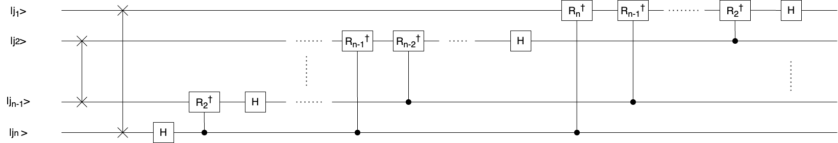
Inverse Quantum Fourier Transformation
Inverse Quantum Fourier Transformation (IQFT) is the inverse operation of QFT. The circuit of IQFT can be constructed by the inverse of the circuit of QFT because each gate in QFT is unitary. The only thing is to reverse the order of gates in QFT and apply conjugates of gates.
\[\begin{align} |j> \xrightarrow{QFT} \frac{1}{\sqrt{N}}\sum_{k=0}^{N-1}e^{\frac{2i\pi jk}{N}}|k> \xrightarrow{IQFT} |j> \\ \end{align} \]
We need to know \(R_{k}^{\dagger}\) is the conjugates of \(R_{k}\),
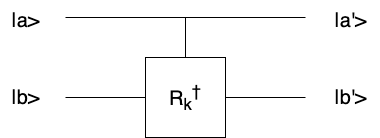
\[CR_k^{\dagger} = \begin{pmatrix} 1 & 0 & 0 & 0 \\ 0 & 1 & 0 & 0 \\ 0 & 0 & 1 & 0 \\ 0 & 0 & 0 & e^{-\frac{2i\pi}{2^k}} \end{pmatrix} \]
When the input |a> and |b>,
\[\begin{align} |b'> &= e^{-\frac{2i\pi a}{2^k}}|b> = e^{-2i\pi 0.\overbrace{00\cdots0}^{k-1}a}|b> \\ \end{align} \]
When the input |j> = \(|j_1 j_2 \cdots j_n>\), the IQFT of |j> as follows
\[ \frac{1}{\sqrt{N}} (|0> + e^{-2i\pi 0.j_{n}}|1>)(|0> + e^{-2i\pi 0.j_{n-1}j_{n}}|1>)\cdots (|0> + e^{-2i\pi 0.j_1j_2\cdots j_{n}}|1>) \]