Variational Quantum Eigenvalue is a classical and quantum algorithm, which uses classical and quantum computers to find the ground state energy of a Hamiltonian.
In quantum part:
1. Ansatz: a parameterized quantum circuit is constructed to generate quantum states.
2. Measurement: these measurement on quantum states is used to estimate the expectation value of the Hamiltonian.
In classical part:
Classical optimization: the primary objective is to minimize the expectation value from quantum measurements. The optimization process involves iteratively refining the parameters of the ansatz and then the expectation value of the Hamiltonian obtained through quantum measurements is minimized. This iterative refinement of the parameters continues until the ground state energy is obtained or a convergence criterion is met. The classical optimization uses gradient descent, stochastic gradient descent, or others, to adjust the parameters of the ansatz.
Explanation:
A Hamiltonian can be presented by a Hermitian matrix. For a matrix H, it satisfied the property:
\[ H = H^{\dagger}\]
where \(H^{\dagger}\) denotes the conjugate transpose of H.
We suppose \(\mu_i \text{ and } \lambda_i \) are one eigenvector and eigenvalue of the matrix H. Then,
\[ H\mu_i = \lambda_i\mu_i \]
We can see the eigenvector as a quantum state \(|\mu_i>\), then,
\[H|\mu_i> = \lambda_i|\mu_i>\]
\[\lambda_i = <\mu_i|H|\mu_i>\]
The target of VQE is to find the lowest eigenvalue \(\lambda\) of the matrix H. To achieve this, VQE constructs an ansatz which prepares a quantum state that is a linear combination of certain basis states. This quantum state may not be an exact eigenvector of the matrix H, but it is a superposition of some basis states, each corresponding to an eigenvector of the matrix H. The expectation value of H in the prepared quantum state is then measured using quantum measurements. If the optimization converges to a minimal value, it indicates that the prepared quantum state is close to an eigenvector of the H, and the expectation value is the estimated lowest eigenvalue. \(E_0\) represents the ground energy of H, and \(|\varphi>\) represents the prepared quantum state.
\[E_0 \leqslant \frac{<\varphi|H|\varphi>}{<\varphi|\varphi>} \]
The key of quantum part is how to construct ansatz and measure the expectation value.
We need to know a Hamiltonian can be expressed as a linear combination of Pauli operators
\[H = \sum_{i\alpha}h_{\alpha}^{i}\sigma_{\alpha}^{i} + \sum_{ij\alpha\beta}h_{\alpha\beta}^{ij}\sigma_{\alpha}^{i}\sigma_{\beta}^{j} + \cdot \cdot \cdot \]
where i and j are qubit, and \(\alpha \text{ and } \beta \) represents Pauli operate X, Y or Z. \(\alpha \in \{X, Y, Z\}, \beta \in \{X, Y, Z\}\). \(\sigma_\alpha^i\) represents a X operator acting on the ith qubit when \(\alpha = X\)
Ansatz is used to prepare quantum states. There are some types of ansatz, such as hardware-efficient ansatz, unitary coupled cluster(UCC) ansatz, etc. I can not explain why use these ansatz.
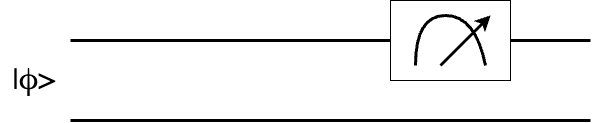
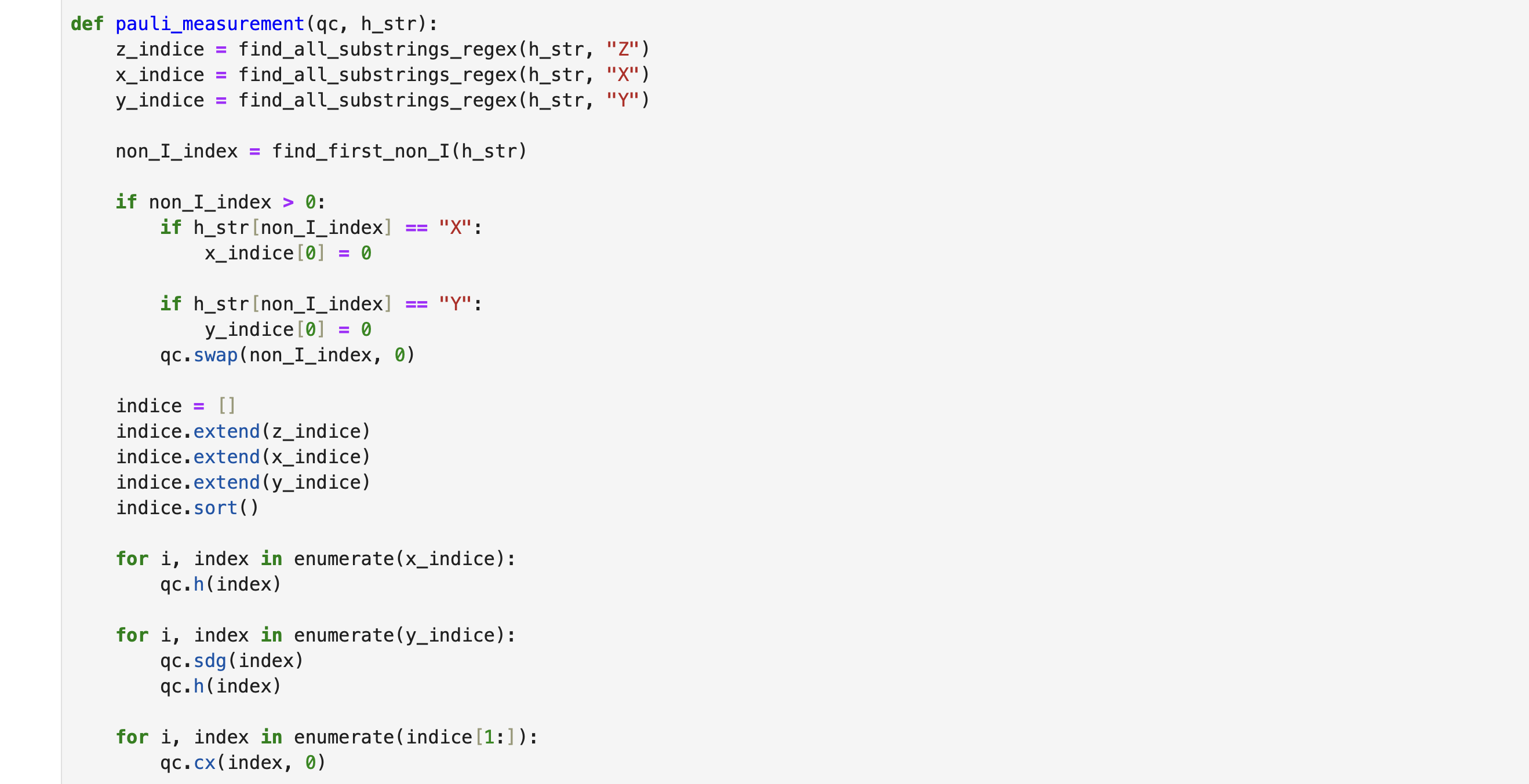
Pauli Measurement
One-qubit Measurement
Pauli Measurement is measurements performed with respect to the Pauli-X(X), Pauli-Y(Y) and Pauli-Z(Z) operator. In VQE, the Pauli-Z measurement is used to estimate the expectation value of the matrix H.
Pauli-Z measurement: it provides the probability of finding the qubit in the |0> or |1> state.
Pauli-X measurement: it provides the probability of finding the quantum state in the |+> or |->.
\[|+> = \frac{|0> + |1>}{\sqrt{2}}\]
\[|-> = \frac{|0> - |1>}{\sqrt{2}}\]
Pauli-Z measurement: it provides the probability of finding the quantum state in the |l> or |r>.
\[|l> = \frac{|0> + i|1>}{\sqrt{2}}\]
\[|r> = \frac{|0> - i|1>}{\sqrt{2}}\]
In VQE, Pauli-Z measurement is used so that I will introduce how to use Pauli-Z measurement to estimate the expectation value of the Pauli-Z operator on one quantum state. Suppose we have the quantum state as follows,
\[|\phi> = \alpha|0> + \beta|1>\]
The expectation value of the Z operator:
\[ <\phi|Z|\phi> = \begin{pmatrix}\alpha & \beta \end{pmatrix}\begin{pmatrix} 1 & 0 \\ 0 & -1 \end{pmatrix} \begin{pmatrix} \alpha \\ \beta \end{pmatrix} = |\alpha|^2 - |\beta|^2 \]
We can see that the expectation of Pauli-Z on one quantum state equals the probability of |0> minus the probability of |1>.
\[<\phi|Z|\phi> = P(0) - P(1)\]
Pauli-X and Pauli-Y operators can be expressed in terms of Pauli-Z operator and unitary operators.
\[X = HZH\]
\[Y = SH Z HS^\dagger\]
Measuring the expectation of the Pauli-X operator on one qubit can follow the method of the Z operator because the X or Y operator can be expressed by the Z operator and quantum gates.
The expectation value of the operator X:
\[<\phi|X|\phi> = <\phi|HZH|\phi>\]
It is easy to note that the expectation of the Pauli-X operator on one quantum state can be obtained with Pauli-Z measurement after the quantum state is applied by a H gate.
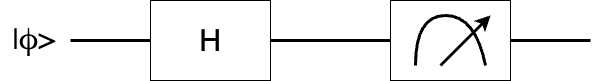
\[\text{Figure 1.1 the quantum circuit of the measurement of the X operator}\]
\[<\phi|X|\phi> = P(0) - P(1)\]
where P(0) and P(1) represent the probability of finding the quantum state in |0> and |1> respectively in the Figure 1.1.
The expectation value of the Y operator:
\[<\phi|Y|\phi> = <\phi|SH Z HS^\dagger|\phi>\]
The expectation of the Pauli-X operator on one quantum state can be obtained with Pauli-Z measurement after the quantum state is applied by a H gate and S gate

\[\text{Figure 1.2 the quantum circuit of the measurement of the Y operator}\]
\[<\phi|Y|\phi> = P(0) - P(1)\]
where P(0) and P(1) represent the probability of finding the quantum state |0> and |1> respectively in the Figure 1.2.
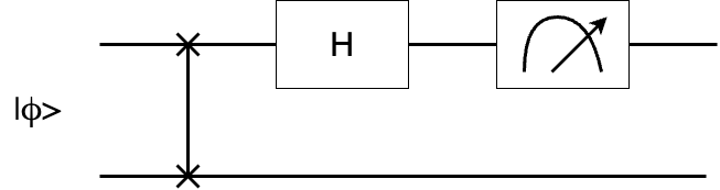
Multiple-qubit measurements
A Hamiltonian normally involves not only single Pauli operators but also the combination of multiple Pauli operators. These combinations can include tensor products of Pauli operators acting on different qubits. It is important to obtain the expectation value of multiple Pauli operators. We take the two-qubit quantum system to measure the expectation value of \(Z \otimes 1 \).
\[|\phi> = \alpha_{00}|00> + \alpha_{01}|01> + \alpha_{10}|10> + \alpha_{11}|11>\]
\[\begin{align} <\phi|Z\otimes 1|\phi> &= \begin{pmatrix} \alpha_{00} & \alpha_{01} & \alpha_{10} & \alpha_{11} \\ \end{pmatrix} \begin{pmatrix} 1 & 0 & 0 & 0 \\ 0 & 1 & 0 & 0 \\ 0 & 0 & -1 & 0 \\ 0 & 0 & 0 & -1 \\ \end{pmatrix} \begin{pmatrix} \alpha_{00} \\ \alpha_{01} \\ \alpha_{10} \\ \alpha_{11} \\ \end{pmatrix} \\ &= |\alpha_{00}|^2 + |\alpha_{01}|^2 - |\alpha_{10}|^2 - |\alpha_{11}|^2 \\ &= P(00) + P(01) - P(10) - P(11) \\ &= P(0) - P(1) \end{align} \]
where P(00), P(01), P(10) and P(11) are the probability of the quantum state |00>, |01>, |10> and |11> respectively, and P(0) and P(1) are the probability of the measurement on the first qubit in the quantum state |0> and |1> respectively. The quantum circuit is as follows,
\[\text{Figure 1.3 the measurement on Z } \otimes 1 \]
According to the approach of the one-qubit system, other operators can be expressed in terms of Z \(\otimes \) 1 and other quantum gates. I list the Pauli measurements on a two-qubit system as the table from reference [1]
\[ \]
| Pauli Measurement | Unitary Operator |
|---|---|
| Z \(\otimes\) 1 | 1 \(\otimes\) 1 |
| X \(\otimes\) 1 | H \(\otimes\) 1 |
| Y \(\otimes\) 1 | \(HS^\dagger \otimes 1\) |
| 1 \(\otimes\) Z | SWAP |
| 1 \(\otimes\) X | (H \(\otimes\) 1)SWAP |
| 1 \(\otimes\) Y | (\(HS^\dagger \otimes 1\))SWAP |
| Z \(\otimes\) Z | \(CNOT_{10}\) |
| X \(\otimes\) Z | \(CNOT_{10}(H\otimes 1)\) |
| Y \(\otimes\) Z | \(CNOT_{10}{HS^\dagger \otimes 1}\) |
| Z \(\otimes\) X | \(CNOT_{10}(1 \otimes H)\) |
| X \(\otimes\) X | \(CNOT_{10}(H \otimes H)\) |
| Y \(\otimes\) X | \(CNOT_{10}(HS^\dagger \otimes H)\) |
| Z \(\otimes\) Y | \(CNOT_{10}(1 \otimes HS^\dagger)\) |
| X \(\otimes\) Y | \(CNOT_{10}(H \otimes HS^\dagger)\) |
| Y \(\otimes\) Y | \(CNOT_{10}(HS^\dagger \otimes HS^\dagger)\) |
The Figure 1.3 is the fundamental part of a two-qubit Pauli measurement for \(Z \otimes 1\). Other Pauli measurements in the table are expressed in terms of \(Z \otimes 1\). I will take an example as follows,
\[\begin{align} SWAP(H\otimes I)&(Z\otimes I)(H\otimes I)SWAP \\ &=SWAP(X\otimes I)SWAP \\ &=\begin{pmatrix} 1 & 0 & 0 & 0 \\ 0 & 0 & 1 & 0 \\ 0 & 1 & 0 & 1 \\ 0 & 0 & 0 & 1 \\ \end{pmatrix} \begin{pmatrix} 0 & 0 & 1 & 0 \\ 0 & 0 & 0 & 1 \\ 1 & 0 & 0 & 0 \\ 0 & 1 & 0 & 0 \\ \end{pmatrix} \begin{pmatrix} 1 & 0 & 0 & 0 \\ 0 & 0 & 1 & 0 \\ 0 & 1 & 0 & 1 \\ 0 & 0 & 0 & 1 \\ \end{pmatrix} \\ &= \begin{pmatrix} 0 & 1 & 0 & 0 \\ 1 & 0 & 0 & 0 \\ 0 & 0 & 0 & 1 \\ 0 & 0 & 1 & 0 \\ \end{pmatrix} \\ &= I \otimes X \end{align} \]
We can get the expression and the measurement as follows
\[I \otimes X = SWAP(H\otimes I)(Z\otimes I)(H\otimes I)SWAP\]
\[<\phi|(I\otimes X)|\phi> = P(0) - P(1)\]
We take another example \(Z \otimes Z\),
\[\begin{align} &CNOT_{10}(Z \otimes I)CNOT_{10}\\ &=\begin{pmatrix} 1 & 0 & 0 & 0 \\ 0 & 0 & 0 & 1 \\ 0 & 0 & 1 & 0 \\ 0 & 1 & 0 & 0 \\ \end{pmatrix} \begin{pmatrix} 1 & 0 & 0 & 0 \\ 0 & 1 & 0 & 0 \\ 0 & 0 & -1 & 0 \\ 0 & 0 & 0 & -1 \\ \end{pmatrix} \begin{pmatrix} 1 & 0 & 0 & 0 \\ 0 & 0 & 0 & 1 \\ 0 & 0 & 1 & 0 \\ 0 & 1 & 0 & 0 \\ \end{pmatrix} \\ &=\begin{pmatrix} 1 & 0 & 0 & 0 \\ 0 & -1 & 0 & 0 \\ 0 & 0 & -1 & 0 \\ 0 & 0 & 0 & 1 \\ \end{pmatrix}\\ &= Z \otimes Z \end{align} \]
We can get the equation \(Z \otimes Z = CNOT_{10}(Z\otimes I)CNOT_{10}\)
The circuit for measurement as follows,

\[<\phi|(Z\otimes Z)|\phi> = P(0) - P(1)\]
Reader can verify other Pauli measurement by themselves and I do not explain them one by one. Note that we always need to find one expression in terms of \(Z\otimes I\).
I will give the structure of VQE as follows,
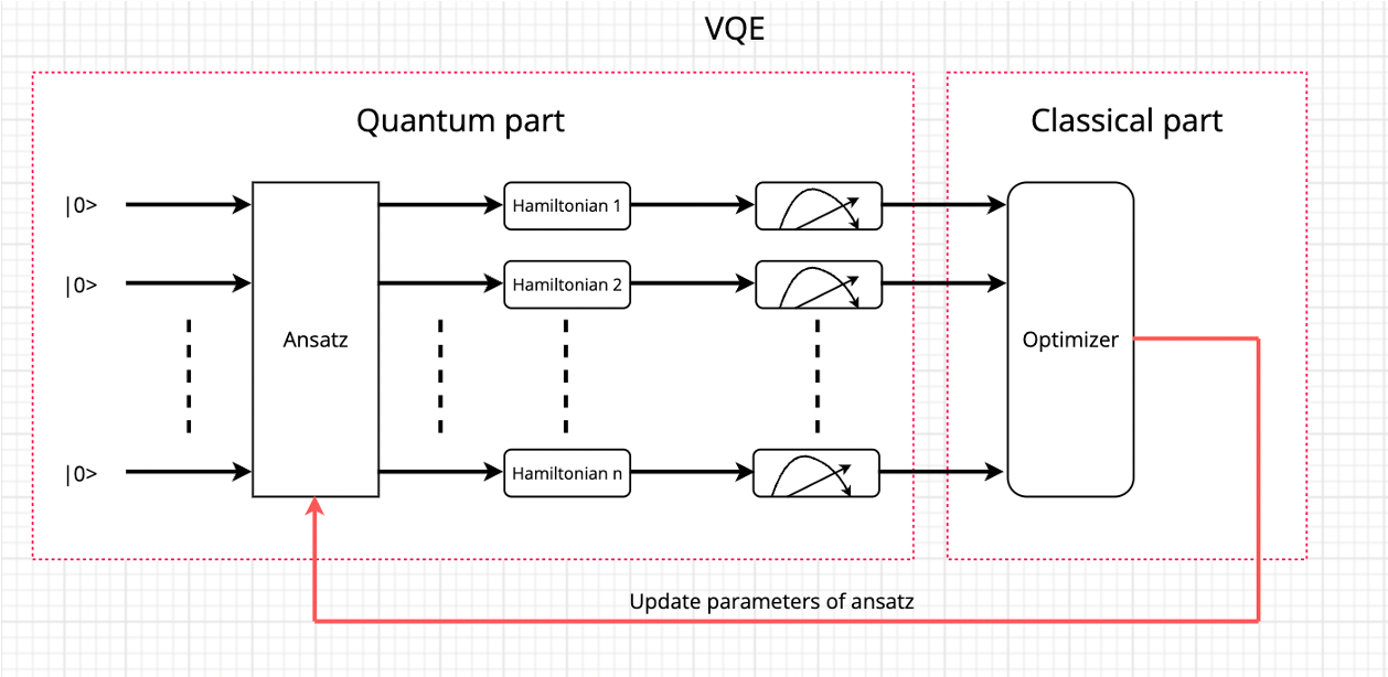
where each hamiltonian can be constructed by Pauli measurements, like Figure 1.1, 1.2 or 1.3.
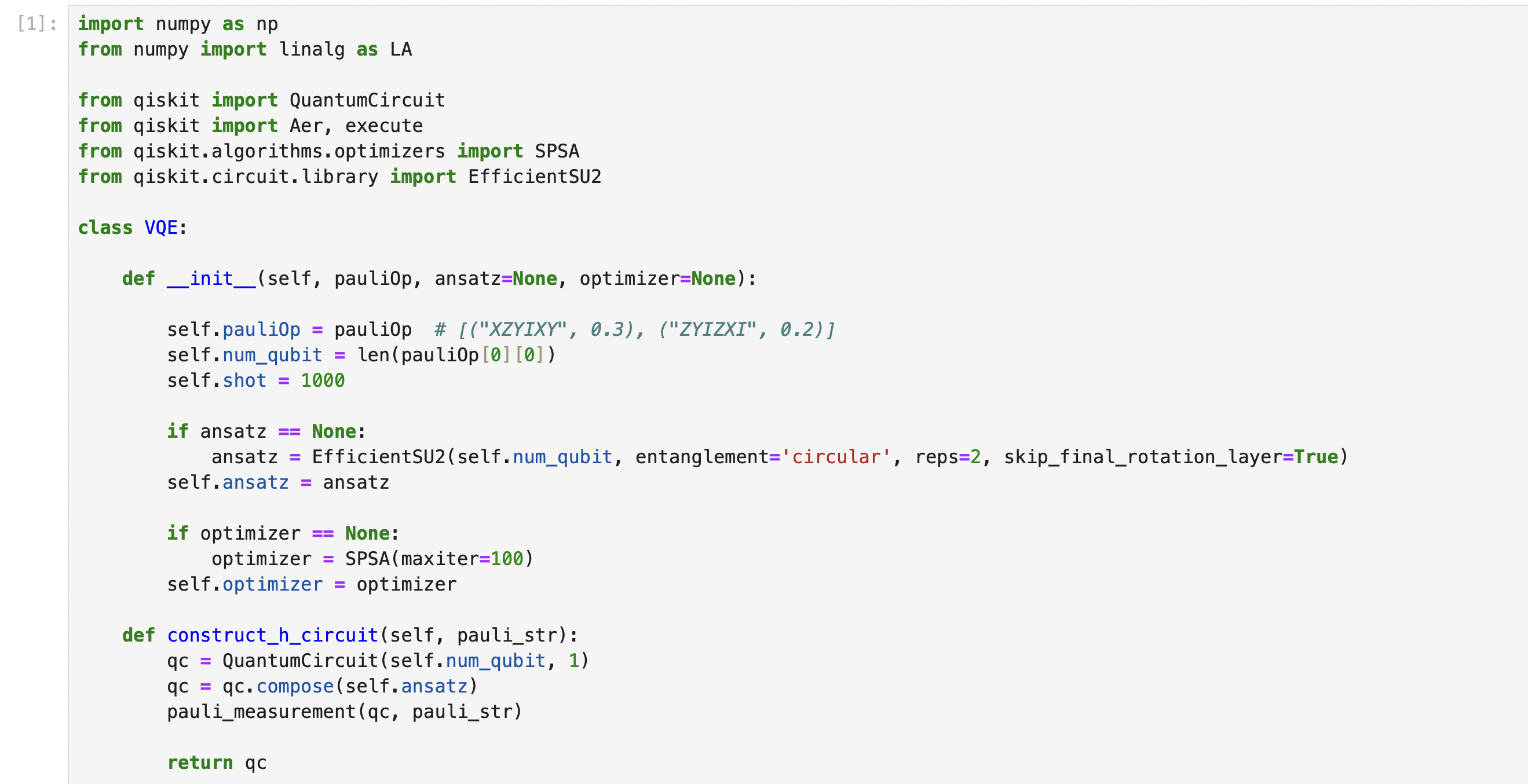
Example on Qiskit
While Qiskit provides a convenient library of VQE, it is beneficial to understand the underlying quantum circuits to appreciate how VQE operates. To illustrate the working of VQE, we construct quantum circuits that represent the key components of VQE. These circuits involve parameterized quantum gates (Ansatz) and pauli measurement. We can measure the expectation value of the Hamiltonian by applying it to the trial state and measuring the resulting energy. The classical optimization SPSA is used to minimize the energy expectation value. This iterative process until convergence. Then we can get the expectation value that approximates the ground value of the Hamiltonian.
Here, we take an example, the Hamiltonian as follows,
\[H = 0.3\times XZYIXY + 0.2\times ZYIZXI\]
We can get the exact lowest eigenvalue of the Hamiltonian through Python3 as follows,
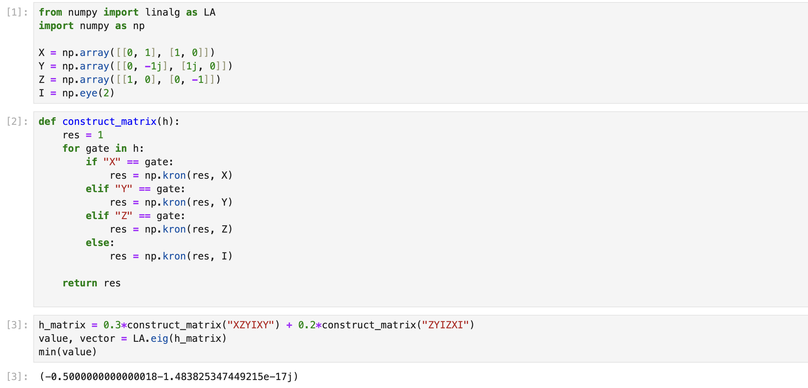
We can see the exact lowest eigenvalue is -0.5.
We can run the VQE on qiskit with classical optimizer that we use SPSA. However, I can not guarantee the final result always equals the exact value because it depends on the optimizer.
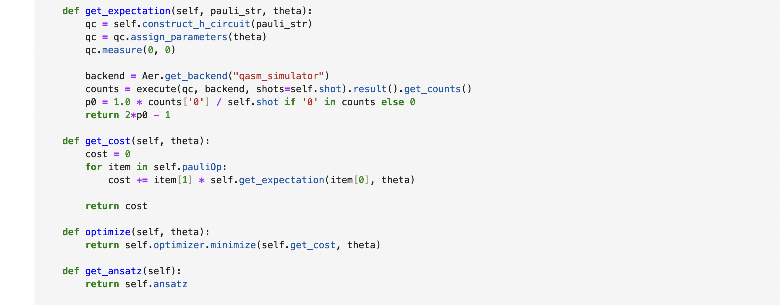
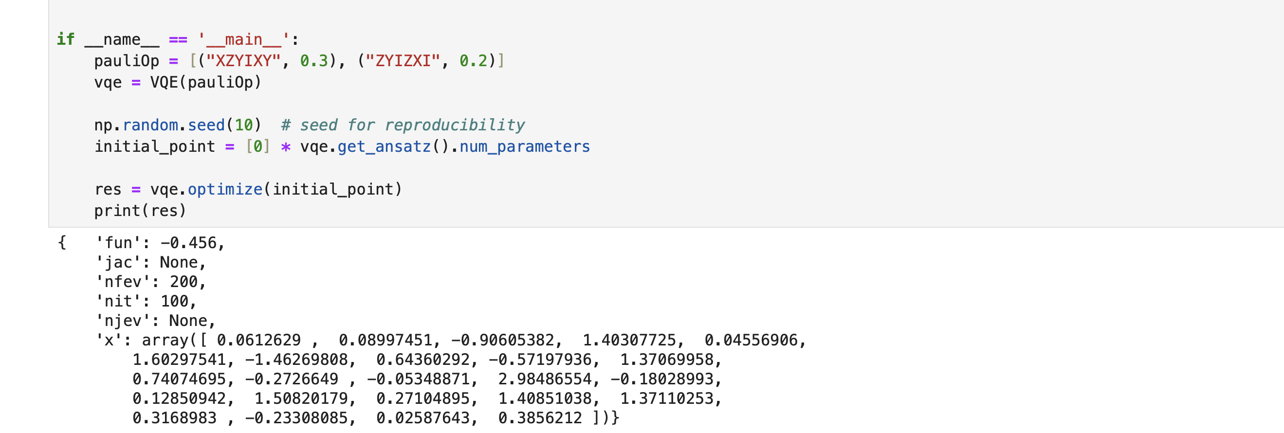
We can see the result is -0.456 from qiskit which is close to the exact value -0.5. It illustrates the VQE is able to find the ground value of a Hamiltonian.
Qiskit version
Qiskit == 0.43.0