Quantum counting is a quantum algorithm for estimating the number of solutions for a given search set. In a search problem, how to quickly determine the number of solutions? In classical computing, it requires the time complexity of O(N), where N represents the length of a search data set. Compared to classical computing, the time complexity of quantum counting is O(\( \sqrt{N} \)). Sometimes the number of solutions are required to be found, and it also is used to decide whether there is a solution in the dataset. Therefore, it is important to introduce the quantum counting algorithm.
Define quantum counting from [1].
\[ f(x) = \begin{cases} 1& x \in B \\ 0& x \notin B \\ \end{cases} \]
B is a set of solutions (that is a subset of \(\{0, 1\}^n\)) and the size of the solution is N = \(2^n\).
The core of the quantum counting algorithm is to estimate the eigenvector of Grover operator. I will explain why we need to use Grover operator. Firstly, we suppose two quantum states which are the same as Grover search:
\[|\alpha> = \frac{1}{\sqrt{N-M}}\sum_{x \notin B}|x>\]
\[|\beta> = \frac{1}{\sqrt{M}}\sum_{x \in B}|x>\]
Where M is the solution of quantum counting.
\[|\Phi> = \frac{1}{\sqrt{N}}\sum_{x=0}^{N-1}|x> = \sqrt{\frac{N-M}{N}}|\alpha> + \sqrt{\frac{M}{N}}|\beta>\]
As we have introduced the Grover operator in Grover's search, the matrix:
\[G = \begin{pmatrix} \cos \theta & -\sin \theta \\ \sin \theta & \cos \theta \\ \end{pmatrix} \]
Note that the \(\theta\) is the angle between \(|\Phi> \text{ and } G|\Phi>\), and also equals the double of the angle between \(|\phi> \text{ and } |\alpha> \).
Now I give the proof of the Grover operator G.
Firstly, calculate the angle between \(|\Phi> \text{ and } |\alpha>\)
\[\cos\frac{\theta}{2} = <\Phi|\alpha> = \sqrt{\frac{N-M}{N}} \]
Then, \[\sin\frac{\theta}{2} = \sqrt{\frac{M}{N}}\]
\[\sin\theta = 2 \sin\frac{\theta}{2}\cos\frac{\theta}{2} = \frac{2\sqrt{M(N-M)}}{N}\]
\[\cos\theta = \frac{N-2M}{N}\]
After applying G on \(|\alpha>\),
\[\begin{align} G|\alpha> &= WV|\alpha> \\ &= (2<\varphi|\varphi> - I)|\alpha> \\ &= 2\sqrt{\frac{N-M}{N}}|\Phi> - |\alpha> \\ &= 2\sqrt{\frac{N-M}{N}}(\sqrt{\frac{N-M}{N}}|\alpha> + \sqrt{\frac{M}{N}}|\beta>) - |\alpha> \\ &= \frac{N-2M}{N}|\alpha> + \frac{2\sqrt{M(N-M)}}{N}|\beta> \\ &= \cos\theta|\alpha> + \sin\theta|\beta> \\ \end{align} \]
After applying G on \(|\beta>\),
\[\begin{align} G|\beta> &= WV|\beta> = (I - 2<\Phi|\Phi>)|\beta> \\ &= |\beta> - 2\sqrt{\frac{M}{N}}|\Phi> \\ &= |\beta> - 2\sqrt{\frac{M}{N}}(\sqrt{\frac{N-M}{N}}|\alpha> + \sqrt{\frac{M}{N}}|\beta>) \\ &= (1 - \frac{2M}{N})|\beta> - \frac{2\sqrt{M(N-M)}}{N}|\alpha> \\ &= -\sin\theta|\alpha> + \cos\theta|\beta> \\ \end{align} \]
\(|\alpha> \text{ and } \beta> \) is a group of orthogonal vectors as orthogonal basis of the operator G,
We can suppose the matrix of G, \(<\alpha| = [1, 0] \text{ and } <\beta| = [0, 1]\)
\[G = \begin{pmatrix} A & B \\ C & D \\ \end{pmatrix} \]
\[G|\alpha> = \begin{pmatrix} A & B\\ C & D \\ \end{pmatrix} \begin{pmatrix} 1 \\ 0\\ \end{pmatrix} = \begin{pmatrix} A \\ C \\ \end{pmatrix} = A|\alpha> + C|\beta> \]
Then, we can get
\[ A = \cos\theta\]
\[ C = \sin\theta\]
\[ G|\beta> = \begin{pmatrix} A & B \\ C & D \\ \end{pmatrix} \begin{pmatrix} 0 \\ 1 \\ \end{pmatrix} = \begin{pmatrix} B \\ D \\ \end{pmatrix} = B|\alpha> + D|\beta>\]
Then, we can get,
\[ B = -\sin\theta\]
\[ D = \cos\theta\]
This is the proof of the operator G.
When we know the matrix of the operator G, it is easy to know the eigenvalue of G is \(e^{\pm i\theta}\). Also, we know,
\[\sin(\frac{\theta}{2}) = \sqrt{\frac{M}{N}}\]
When we estimate the eigenvalue of G, it is easy to get the value of M = \(N\sin^2{\frac{\theta}{2}}\).
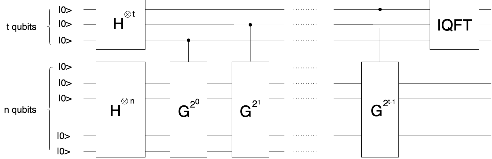
The circuit consists of two registers, one has t qubits and the other has n qubits. It is as follows
Example on Qiskit
The Grover operator is from Grover's search. The search range is {000, 001, 010, 011, 100, 101, 110, 111} and the targets are 011 and 110 so the number of solutions is 2.


